Chapter 3 Google Capstone [DA|R]
In my free time, I audited the Google Data Analytics courses and completed its capstone.
3.1 Description
Performed data analysis for a fictional bike-share company to illustrate the data analysis process learned from the Google Data Analytics Professional Certificate:
- Ask: Business objective, questions, challenges
- Prepare: Data generation, collection, storage, and management
- Process Data cleaning, ensuring data integrity
- Analyze: Data exploration, finding patterns/trends
- Share: Interpreting and communicating results
- Act: Using insights to solve the problem
3.1.1 Scenario
Cyclistic’s director of marketing believes the company’s future success depends on maximizing the number of annual memberships. Customers who purchase single-ride or full-day passes are referred to as casual riders.
- Your team wants to understand how casual riders and annual members use Cyclistic bikes differently
From these insights, a new marketing strategy will be designed to convert casuals into members.
3.2 Ask
Three questions will guide the future marketing program. The director assigned me the first:
- How do annual members and casual riders use Cyclistic bikes differently?
- Why would casual riders buy Cyclistic annual memberships?
- How can Cyclistic use digital media to influence casual riders to become members?
The task is to produce a report with the following deliverables:
- A clear statement of the business task
- A description of all data sources and software used
- Documentation of any cleaning or manipulation of data
- A summary of the analysis
- Supporting visualizations and key findings
- Recommendations based on analysis
3.3 Prepare / Process
The (fictional) historical data, divvy-tripdata, is publicly available and hosted on AWS.
I used the Amazon Web Services Command Line Interface (AWS CLI) to scrape a year’s worth of data (August 2021 - July 2022 inclusive):
#!/bin/zsh
# Bucket name is simply from url: <bucket_name>.s3.amazonaws.com
# First exclude all objects, then include those needed
# This will download the files into current directory, then unzip and rm zip
aws s3 sync s3://divvy-tripdata . \
    --exclude '*' \
    --include '20210[8-9]*.zip' \
    --include '20211[0-2]*.zip' \
    --include '20220[1-7]*.zip' \
&& unzip '*.zip' && rm *.zip && rm -rf __MACOSX/
I baked the following packages into some boilerplate code, then defined any necessary functions for pre-processing:
packages <- c("tidyverse", "here", "skimr", "janitor", "Hmisc", "geosphere",
              "sjmisc", "lubridate", "scales", "RColorBrewer", "ggmap", "gridExtra")

for (package in packages) {
  if (!require(package, character.only = TRUE)) {
    print("Installing package(s)")
    install.packages(package, repos = "http://cran.us.r-project.org")
    library(package, character.only = TRUE)
    if (require(package, character.only = TRUE)) {
      print("Package(s) installed and loaded")
    } else {
      stop("Could not install package(s)")
    }
  }
}

# dplyr case_when + factors
fct_case_when <- function(...) {
  args <- as.list(match.call())
  levels <- sapply(args[-1], function(f) f[[3]])  # extract RHS of formula
  levels <- levels[!is.na(levels)]
  factor(case_when(...), levels=levels)
}
3.3.1 Pre-Processing with R
My workflow to ensure the data’s integrity; cleaning and formatting it such that it’s ready for analysis:
# Store names of the files in list, path = . (default)
files = list.files(pattern = "*tripdata.csv")

# Use those names to read in the csvs and properly rename them
bike_data_raw <- lapply(files, read_csv, show_col_types = FALSE) %>%
                 setNames(paste0(substring(files,1,6), "_bike_data"))

# Convert relevant data to factors and merge list into a single dataframe
bike_data_raw <- bike_data_raw %>%
                   lapply(mutate,
                          member_casual = as.factor(str_to_title(member_casual)),
                          rideable_type = as.factor(rideable_type)) %>%
bind_rows()glimpse(bike_data_raw)## Rows: 5,901,463
## Columns: 13
## $ ride_id <chr> "99103BB87CC6C1BB", "EAFCCCFB0A3FC5A1", "9EF4F46C57…
## $ rideable_type <fct> electric_bike, electric_bike, electric_bike, electr…
## $ started_at <dttm> 2021-08-10 17:15:49, 2021-08-10 17:23:14, 2021-08-…
## $ ended_at <dttm> 2021-08-10 17:22:44, 2021-08-10 17:39:24, 2021-08-…
## $ start_station_name <chr> NA, NA, NA, NA, NA, NA, NA, NA, NA, NA, NA, NA, NA,…
## $ start_station_id <chr> NA, NA, NA, NA, NA, NA, NA, NA, NA, NA, NA, NA, NA,…
## $ end_station_name <chr> NA, NA, NA, NA, NA, NA, NA, "Clark St & Grace St", …
## $ end_station_id <chr> NA, NA, NA, NA, NA, NA, NA, "TA1307000127", NA, NA,…
## $ start_lat <dbl> 41.77000, 41.77000, 41.95000, 41.97000, 41.79000, 4…
## $ start_lng <dbl> -87.68000, -87.68000, -87.65000, -87.67000, -87.600…
## $ end_lat <dbl> 41.77000, 41.77000, 41.97000, 41.95000, 41.77000, 4…
## $ end_lng <dbl> -87.68000, -87.63000, -87.66000, -87.65000, -87.620…
## $ member_casual <fct> Member, Member, Member, Member, Member, Member, Mem…# Columns containing NAs
colnames(bike_data_raw)[colSums(is.na(bike_data_raw)) > 0]## [1] "start_station_name" "start_station_id" "end_station_name"
## [4] "end_station_id" "end_lat" "end_lng"# Drop NA
bike_data_raw <- drop_na(bike_data_raw)
# Check if there are duplicate ride_IDs
if(n_distinct(bike_data_raw$ride_id) != nrow(bike_data_raw)) {
# Remove duplicate rows
bike_data_raw <- bike_data_raw %>%
distinct(ride_id, .keep_all = TRUE)
}
# Extract columns containing character vectors
tmp_char_cols <- bike_data_raw[, sapply(bike_data_raw, class) == 'character']
colnames(tmp_char_cols)## [1] "ride_id" "start_station_name" "start_station_id"
## [4] "end_station_name" "end_station_id"# Find which rows are test rows
tmp_test_rows <- which(
rowSums(
`dim<-`(grepl("TEST|TESTING", as.matrix(tmp_char_cols)),
dim(tmp_char_cols))
) > 0
)
# View and confirm (subsetted by id for example)
unique(tmp_char_cols[tmp_test_rows, 'end_station_id'])## # A tibble: 344 × 1
## end_station_id
## <chr>
## 1 Hubbard Bike-checking (LBS-WH-TEST)
## 2 13073
## 3 18067
## 4 637
## 5 TA1307000159
## 6 13132
## 7 TA1309000032
## 8 13434
## 9 TA1305000041
## 10 13256
## # … with 334 more rows# Store clean data and clean workspace
bike_data <- bike_data_raw[-tmp_test_rows, ]
rm(files, bike_data_raw, list = ls(pattern='^tmp_'))
glimpse(bike_data)## Rows: 4,628,134
## Columns: 13
## $ ride_id <chr> "DD06751C6019D865", "79973DC3B232048F", "0249AD4B25…
## $ rideable_type <fct> classic_bike, classic_bike, classic_bike, classic_b…
## $ started_at <dttm> 2021-08-08 17:21:26, 2021-08-27 08:53:52, 2021-08-…
## $ ended_at <dttm> 2021-08-08 17:25:37, 2021-08-27 09:18:29, 2021-08-…
## $ start_station_name <chr> "Desplaines St & Kinzie St", "Larrabee St & Armitag…
## $ start_station_id <chr> "TA1306000003", "TA1309000006", "13157", "13042", "…
## $ end_station_name <chr> "Kingsbury St & Kinzie St", "Michigan Ave & Oak St"…
## $ end_station_id <chr> "KA1503000043", "13042", "13157", "13042", "13042",…
## $ start_lat <dbl> 41.88872, 41.91808, 41.87773, 41.90096, 41.90096, 4…
## $ start_lng <dbl> -87.64445, -87.64375, -87.65479, -87.62378, -87.623…
## $ end_lat <dbl> 41.88918, 41.90096, 41.87773, 41.90096, 41.90096, 4…
## $ end_lng <dbl> -87.63851, -87.62378, -87.65479, -87.62378, -87.623…
## $ member_casual <fct> Member, Member, Member, Casual, Casual, Casual, Cas…3.3.2 Feature Engineering
I used the geosphere package (Hijmans 2021) to compute the distance between starting and ending coordinates and implemented lubridate (Spinu, Grolemund, and Wickham 2021) to parse starting dates of trips into buckets. The previously defined function fct_case_when() allows me to further classify the month bucket into factors.
# Features for data integrity: trip_distance (miles), speed (mph)
# The rest are engineered for deeper analysis
bike_data <- bike_data %>%
               mutate(trip_duration = as.numeric(difftime(ended_at, started_at, units = "hours")),
                      trip_distance = distHaversine(cbind(start_lng, start_lat),
                                                    cbind(end_lng, end_lat))/1609.35,
                              speed = trip_distance/trip_duration,
                          trip_hour = hour(started_at),
                           trip_day = wday(started_at, label = TRUE),
                         trip_month = month(started_at, label = TRUE),
                          afternoon = trip_hour %in% seq(12,18),
                            weekend = as.integer(trip_day) %in% c(1, 6, 7),
                             season = fct_case_when(as.integer(trip_month) %in% c(12, 1, 2) ~ "Winter",
                                                    as.integer(trip_month) %in% seq(3, 5)   ~ "Spring",
                                                    as.integer(trip_month) %in% seq(6, 8)   ~ "Summer",
                                                    as.integer(trip_month) %in% seq(9, 11)  ~ "Fall"),
                              route = paste(start_station_name, end_station_name, sep = " to ")
                     )

# Data verification: Are there any immediately "impossible" outliers?
#                    - nonpositive trip durations and extreme speeds
# Caveats: speed = dist/time used, idea is to appromixate the beeline
#          speed one must go to reach destination in given time
#          and compare to max speed possible on bike (~30 mph),
#          instead of an accurate formula & general model which
#          takes into account location, stops, turns, etc.
glimpse(bike_data %>%
          select(trip_distance, trip_duration, speed) %>%
          filter(speed >= 30 | trip_duration <= 0))
## Rows: 721
## Columns: 3
## $ trip_distance <dbl> 0.000000000, 0.000000000, 0.000000000, 0.025981785, 0.00…
## $ trip_duration <dbl> -0.0100000000, 0.0000000000, 0.0000000000, 0.0005555556,…
## $ speed <dbl> 0.0000000, NaN, NaN, 46.7672134, -0.0793921, NaN, NaN, 0…bike_data <- bike_data %>%
filter(speed < 30) %>%
filter(trip_duration > 0)
glimpse(bike_data)## Rows: 4,627,413
## Columns: 23
## $ ride_id <chr> "DD06751C6019D865", "79973DC3B232048F", "0249AD4B25…
## $ rideable_type <fct> classic_bike, classic_bike, classic_bike, classic_b…
## $ started_at <dttm> 2021-08-08 17:21:26, 2021-08-27 08:53:52, 2021-08-…
## $ ended_at <dttm> 2021-08-08 17:25:37, 2021-08-27 09:18:29, 2021-08-…
## $ start_station_name <chr> "Desplaines St & Kinzie St", "Larrabee St & Armitag…
## $ start_station_id <chr> "TA1306000003", "TA1309000006", "13157", "13042", "…
## $ end_station_name <chr> "Kingsbury St & Kinzie St", "Michigan Ave & Oak St"…
## $ end_station_id <chr> "KA1503000043", "13042", "13157", "13042", "13042",…
## $ start_lat <dbl> 41.88872, 41.91808, 41.87773, 41.90096, 41.90096, 4…
## $ start_lng <dbl> -87.64445, -87.64375, -87.65479, -87.62378, -87.623…
## $ end_lat <dbl> 41.88918, 41.90096, 41.87773, 41.90096, 41.90096, 4…
## $ end_lng <dbl> -87.63851, -87.62378, -87.65479, -87.62378, -87.623…
## $ member_casual <fct> Member, Member, Member, Casual, Casual, Casual, Cas…
## $ trip_duration <dbl> 0.069722222, 0.410277778, 0.010277778, 0.078333333,…
## $ trip_distance <dbl> 0.307632959, 1.568416347, 0.000000000, 0.000000000,…
## $ speed <dbl> 4.412265551, 3.822815741, 0.000000000, 0.000000000,…
## $ trip_hour <int> 17, 8, 12, 16, 15, 10, 23, 22, 18, 13, 21, 11, 18, …
## $ trip_day <ord> Sun, Fri, Sun, Thu, Mon, Mon, Sat, Fri, Mon, Thu, W…
## $ trip_month <ord> Aug, Aug, Aug, Aug, Aug, Aug, Aug, Aug, Aug, Aug, A…
## $ afternoon <lgl> TRUE, FALSE, TRUE, TRUE, TRUE, FALSE, FALSE, FALSE,…
## $ weekend <lgl> TRUE, TRUE, TRUE, FALSE, FALSE, FALSE, TRUE, TRUE, …
## $ season <fct> Summer, Summer, Summer, Summer, Summer, Summer, Sum…
## $ route <chr> "Desplaines St & Kinzie St to Kingsbury St & Kinzie…3.4 Analyze
The following is a “slideshow” of relevant statistics and visuals along with their code.
To keep it clean, key observations are listed afterward (with cross-references) in the final report. In normal reports or slideshows, the graphic wouldn’t have the code attached to it – just the caption and key observation(s).
3.4.1 Basic Descriptive Statistics
bike_data %>%
  select(start_lat:end_lng, member_casual:trip_hour) %>%
  group_by(member_casual) %>%
  descr(show = c("mean", "sd", "trimmed", "range", "iqr", "skew"))
##
## ## Basic descriptive statistics
##
##
## Grouped by: Casual
##
## var mean sd trimmed range iqr skew
## start_lat 41.90 0.04 41.90 0.42 (41.65-42.06) 0.04451399 -0.36
## start_lng -87.64 0.03 -87.64 0.3 (-87.83--87.53) 0.02905797 -0.85
## end_lat 41.90 0.04 41.90 0.52 (41.65-42.17) 0.04566567 -0.37
## end_lng -87.64 0.03 -87.64 0.3 (-87.83--87.53) 0.03058697 -0.84
## trip_duration 0.44 1.77 0.31 693.82 (0-693.82) 0.31944444 161.70
## trip_distance 1.36 1.23 1.19 19.85 (0-19.85) 1.20339742 2.19
## speed 5.03 3.14 4.97 29.44 (0-29.44) 4.49007265 0.09
## trip_hour 14.57 5.05 14.95 23 (0-23) 6.00000000 -0.77
##
##
## Grouped by: Member
##
## var mean sd trimmed range iqr skew
## start_lat 41.90 0.04 41.90 0.42 (41.65-42.06) 0.04698683 -0.15
## start_lng -87.65 0.02 -87.64 0.3 (-87.83--87.53) 0.02757026 -0.51
## end_lat 41.90 0.04 41.90 0.42 (41.65-42.06) 0.04708300 -0.15
## end_lng -87.65 0.02 -87.64 0.3 (-87.83--87.53) 0.02757026 -0.52
## trip_duration 0.21 0.29 0.18 24.88 (0-24.88) 0.17111111 31.47
## trip_distance 1.27 1.11 1.09 17.1 (0-17.1) 1.11475723 2.05
## speed 6.71 2.76 6.81 29.98 (0-29.98) 3.09570863 -0.23
## trip_hour 13.94 4.92 14.13 23 (0-23) 8.00000000 -0.433.4.2 Viz: Trip Behavior
I used the RColorBrewer package (Neuwirth 2022) for palettes.
# Pie chart: member vs. casual
bike_data %>%
  select(member_casual) %>%
  group_by(member_casual) %>%
  count() %>%
  ungroup %>%
  mutate(perc = percent(n/sum(n))) %>%
  ggplot(aes(x = "", y = n, fill = member_casual)) +
    geom_bar(stat = "identity", size = 0.25, color = "black", position = "fill") +
    coord_polar(theta = "y") +
    geom_text(aes(label = perc), size = 5, position = position_fill(vjust = 0.5)) +
    theme_void() +
    labs(title = "Casual Riders vs. Annual Members") +
    theme(legend.title = element_blank(), legend.position = "bottom",
          legend.key.size = unit(0.65, "cm"), legend.text = element_text(size = 12),
          plot.title = element_text(color = "black", size = 22, hjust = 0.5))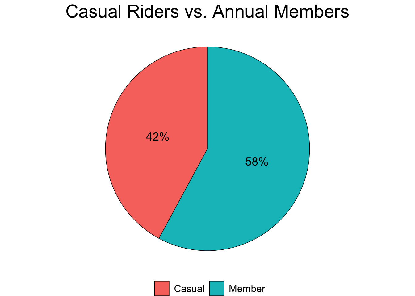
Figure 3.1: Membership Status
# Bar chart: member vs. casual, days of week
bike_data %>%
  select(member_casual, trip_day) %>%
  group_by(member_casual, trip_day) %>%
  count(trip_day) %>%
  ggplot(aes(x = trip_day, y = n, fill = member_casual)) +
    geom_col() +
    facet_wrap( ~member_casual, ncol = 1) +
    scale_y_continuous(labels = comma) +
    labs(title = "Trip Behavior: Days of the Week",
         x = "\nTrip Day", y = "Number of Rides\n") +
    theme(legend.title = element_blank(), legend.key.size = unit(0.65, "cm"),
          legend.text = element_text(size = 12),
          plot.title = element_text(color = "black", size = 22))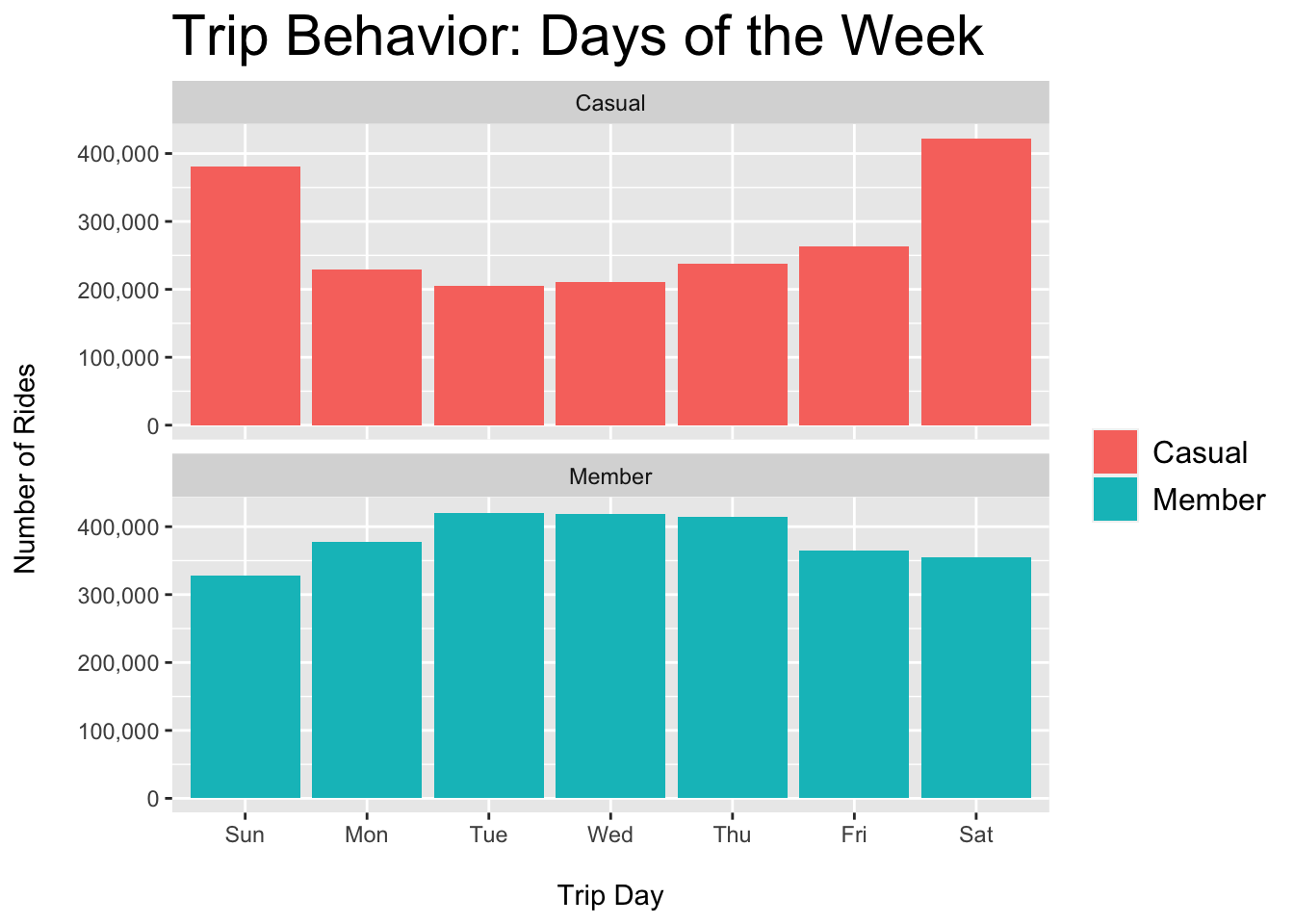
Figure 3.2: Casual vs. Member - Rides per Day
# Pie chart: weekend/weekday use
bike_data %>%
  select(member_casual, weekend) %>%
  group_by(member_casual) %>%
  count(weekend) %>%
  mutate(perc = percent(n/sum(n))) %>%
  ggplot(aes(x = "", y = n, fill = weekend)) +
    geom_bar(stat = "identity", size = 0.25, color = "black", position = "fill") +
    coord_polar(theta = "y") +
    facet_wrap( ~ member_casual) +
    geom_text(aes(label = perc), position = position_fill(vjust = 0.5)) +
    theme_void() +
    scale_fill_manual(values = c("#FBB4AE","#7FC97F")) +
    labs(title = "Weekend Use\n") +
    theme(legend.title = element_blank(), legend.position = "bottom",
          legend.key.size = unit(0.65, "cm"), legend.text = element_text(size = 12),
          strip.text.x = element_text(size = 14),
          plot.title = element_text(color = "black", size = 22, hjust = 0.5))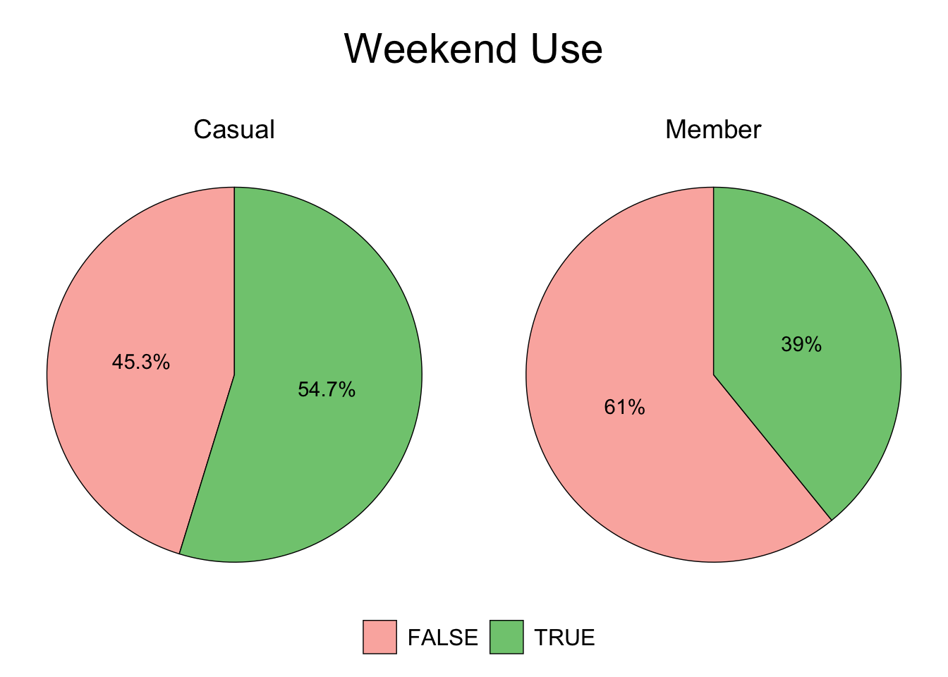
Figure 3.3: Casual vs. Member - Weekend
# Bar chart: member vs. casual, rides by month
bike_data %>%
  select(member_casual, trip_month) %>%
  group_by(member_casual, trip_month) %>%
  count(trip_month) %>%
  ggplot(aes(x = trip_month, y = n, fill = member_casual)) +
    geom_col() +
    scale_y_continuous(labels = comma) +
    labs(title = "Trip Behavior: Months of the Year",
         x = "\nTrip Month", y = "Number of Rides\n") +
    theme(legend.title = element_blank(), legend.key.size = unit(0.65, "cm"),
          legend.text = element_text(size = 12),
          plot.title = element_text(color = "black", size = 22))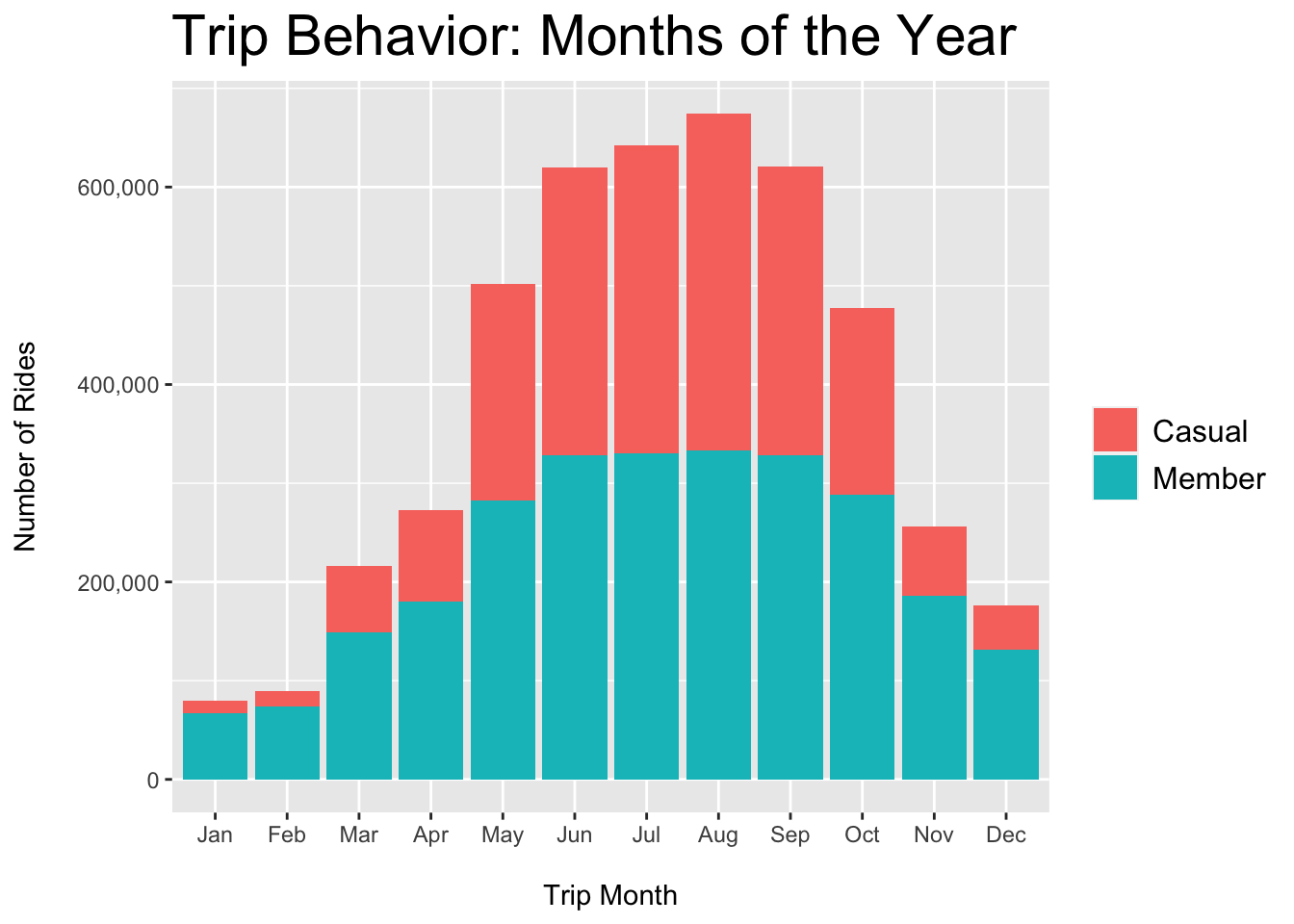
Figure 3.4: Casual vs. Member - Rides per Month
# Pie Chart: member vs. casual, summer use
bike_data %>%
  select(member_casual, season) %>%
  group_by(member_casual) %>%
  count(summer = season == "Summer") %>%
  mutate(perc = percent(n/sum(n))) %>%
  ggplot(aes(x = "", y = n, fill = summer)) +
    geom_bar(stat = "identity", size = 0.25, color = "black", position = "fill") +
    coord_polar(theta = "y") +
    facet_wrap( ~ member_casual) +
    geom_text(aes(label = perc), position = position_fill(vjust = 0.5)) +
    theme_void() +
    scale_fill_manual(values = c("#FBB4AE","#7FC97F")) +
    labs(title = "Summer Use\n") +
    theme(legend.title = element_blank(), legend.position = "bottom",
          legend.key.size = unit(0.65, "cm"), legend.text = element_text(size = 12),
          strip.text.x = element_text(size = 14),
          plot.title = element_text(color = "black", size = 22, hjust = 0.5))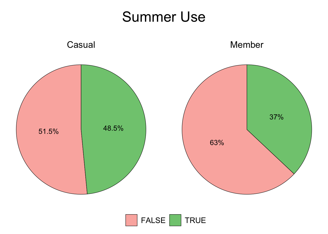
Figure 3.5: Casual vs. Member - Summer
# Bar chart: member vs. casual, rides by hour (total)
bike_data %>%
  select(member_casual, trip_hour) %>%
  group_by(member_casual) %>%
  count(trip_hour) %>%
  ggplot(aes(x = trip_hour, y = n, fill = member_casual)) +
    geom_col() +
    scale_y_continuous(labels = comma) +
    scale_x_continuous(breaks = seq(0, 23)) +
    labs(title = "Trip Behavior: Rides by Hour",
         x = "\nTrip Hour", y = "Number of Rides\n") +
    theme(legend.title = element_blank(), legend.key.size = unit(0.5, "cm"),
          legend.text = element_text(size = 10),
          plot.title = element_text(color = "black", size = 22))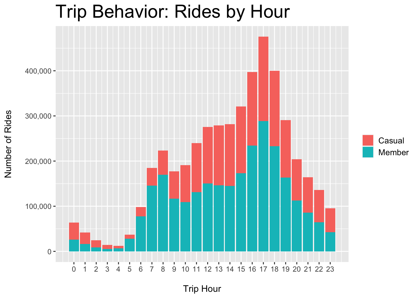
Figure 3.6: Casual vs. Member - Rides per Hour
# Pie chart: member vs casual, afternoon use (12-6 pm)
bike_data %>%
  select(member_casual, afternoon) %>%
  group_by(member_casual) %>%
  count(afternoon) %>%
  mutate(perc = percent(n/sum(n))) %>%
  ggplot(aes(x = "", y = n, fill = afternoon)) +
    geom_bar(stat = "identity", size = 0.25, color = "black", position = "fill") +
    coord_polar(theta = "y") +
    facet_wrap( ~ member_casual) +
    geom_text(aes(label = perc), position = position_fill(vjust = 0.5)) +
    theme_void() +
    scale_fill_manual(values = c("#FBB4AE","#7FC97F")) +
    labs(title = "Afternoon Use\n") +
    theme(legend.title = element_blank(), legend.position = "bottom",
          legend.key.size = unit(0.65, "cm"), legend.text = element_text(size = 12),
          strip.text.x = element_text(size = 14),
          plot.title = element_text(color = "black", size = 22, hjust = 0.5))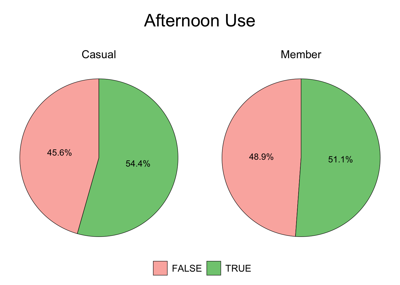
Figure 3.7: Casual vs. Member - Afternoon
# Bar chart: member vs casual, rides by hour (by day)
bike_data %>%
  select(member_casual, trip_day, trip_hour) %>%
  group_by(member_casual, trip_day) %>%
  count(trip_hour) %>%
  ggplot(aes(x = trip_hour, y = n, fill = member_casual)) +
    geom_col() +
    scale_y_continuous(labels = comma) +
    facet_wrap(~ trip_day) +
    labs(title = "Trip Behavior: Rides by Hour", subtitle = "Days of the Week",
         x = "Trip Hour", y = "Number of Rides\n") +
    theme(legend.title = element_blank(), plot.subtitle = element_text(size = 12),
          legend.key.size = unit(0.5, "cm"), legend.text = element_text(size = 10),
          plot.title = element_text(color = "black", size = 22))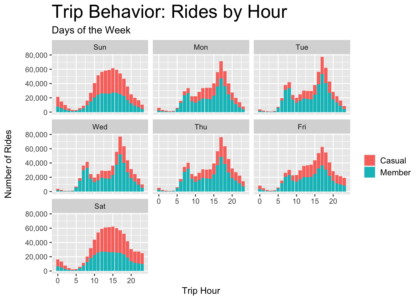
Figure 3.8: Casual vs. Member - Rides per Hour Each Day
# Bar chart: member vs casual, rides by hour (by month)
bike_data %>%
  select(member_casual, trip_month, trip_hour) %>%
  group_by(member_casual, trip_month) %>%
  count(trip_hour) %>%
  ggplot(aes(x = trip_hour, y = n, fill = member_casual)) +
    geom_col() +
    scale_y_continuous(labels = comma) +
    facet_wrap(~ trip_month) +
    labs(title = "Trip Behavior: Rides by Hour", subtitle = "Months of the Year",
         x = "\nTrip Hour", y = "Number of Rides\n") +
    theme(legend.title = element_blank(), plot.subtitle = element_text(size = 12),
          legend.key.size = unit(0.5, "cm"), legend.text = element_text(size = 10),
          plot.title = element_text(color = "black", size = 22))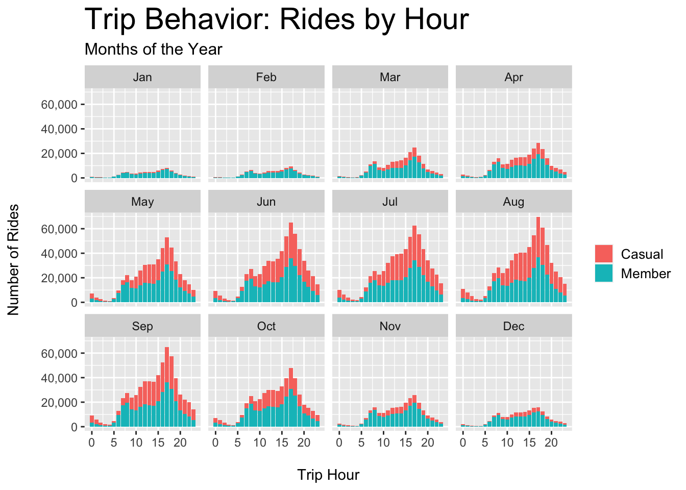
Figure 3.9: Casual vs. Member - Rides per Hour Each Month
# Pie chart by season
bike_data %>%
  select(member_casual, season) %>%
  group_by(member_casual) %>%
  count(season) %>%
  mutate(perc = percent(n/sum(n))) %>%
  ggplot(aes(x = "", y = n, fill = season)) +
    geom_bar(stat = "identity", size = 0.25, color = "black", position = "fill") +
    coord_polar(theta = "y") +
    facet_wrap( ~ member_casual) +
    geom_text(aes(x = 1.675, label = perc), position = position_fill(vjust=0.5),
              size = 3) +
    theme_void() +
    scale_fill_manual(values = c("#C7E9B4", "#7FCDBB", "#41B6C4", "#1D91C0")) +
    labs(title = "Seasonal Use\n") +
    theme(legend.title = element_blank(), legend.position = "bottom",
          legend.key.size = unit(0.65, "cm"), legend.text = element_text(size = 12),
          strip.text.x = element_text(size = 14),
          plot.title = element_text(color = "black", size = 22, hjust = 0.5))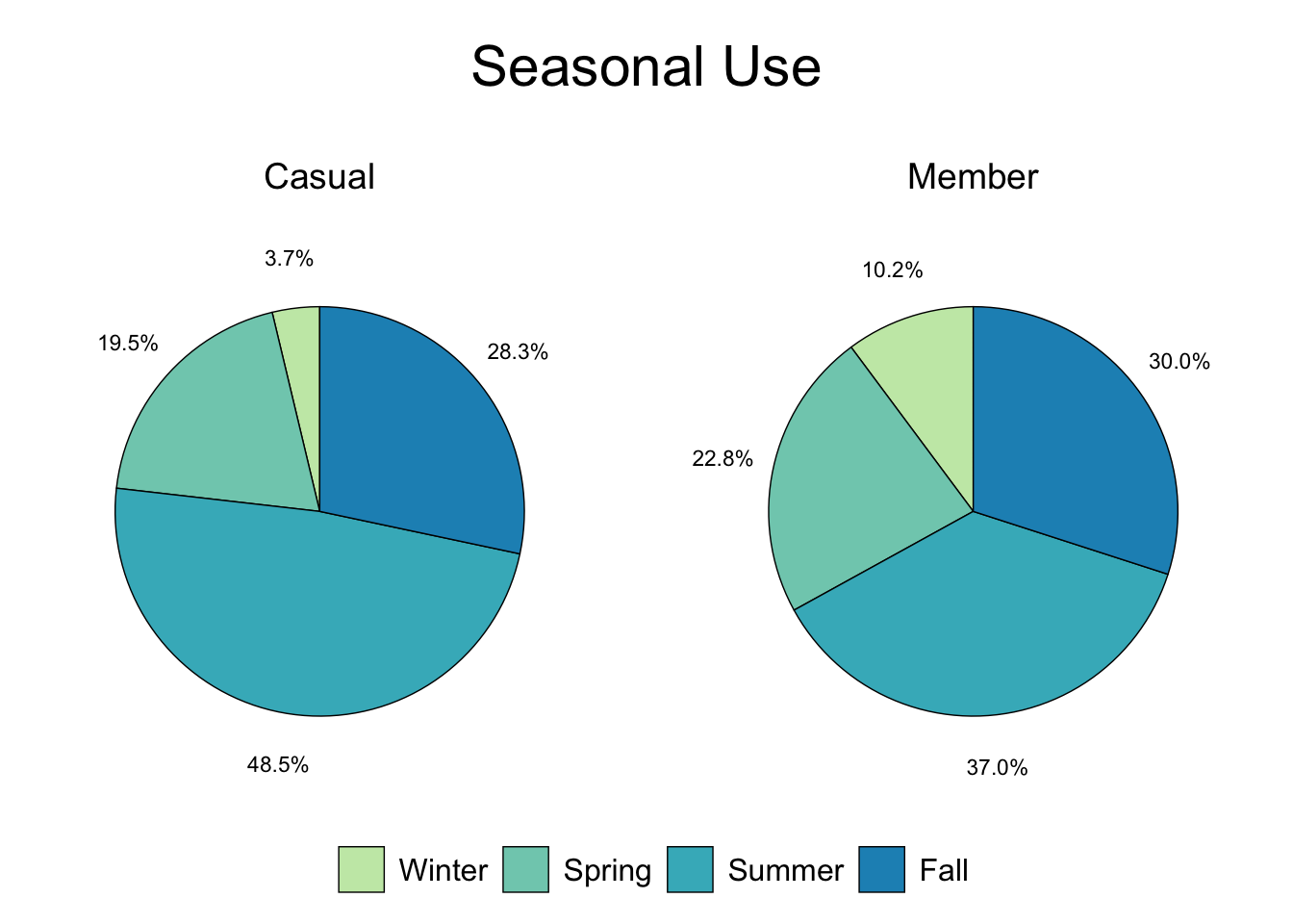
Figure 3.10: Casual vs. Member - Seasons
3.4.3 Viz: Bike Choice
# Pie chart: types of bikes
bike_data %>%
  select(rideable_type) %>%
  count(rideable_type) %>%
  mutate(perc = percent(n/sum(n))) %>%
  ggplot(aes(x = "", y = n, fill = rideable_type)) +
    geom_bar(stat = "identity", size = 0.25, color = "black", position = "fill") +
    coord_polar(theta = "y", direction = -1) +
    geom_text(aes(x = 1.1, label = perc), position = position_fill(vjust = 0.5),
              size = 3.5) +
    theme_void() +
    scale_fill_manual(name = "", values = c("#E5C494", "#B3B3B3", "#FFD92F"),
                      labels = c("Classic", "Docked", "Electric")) +
    labs(title = "Bike Choice (Overall)") +
    theme(legend.title = element_blank(), legend.key.size = unit(0.65, "cm"),
          legend.text = element_text(size = 12), legend.position = "bottom",
          plot.title = element_text(color = "black", size = 22, hjust = 0.5)) +
    guides(fill = guide_legend(reverse = TRUE, title.position = "top"))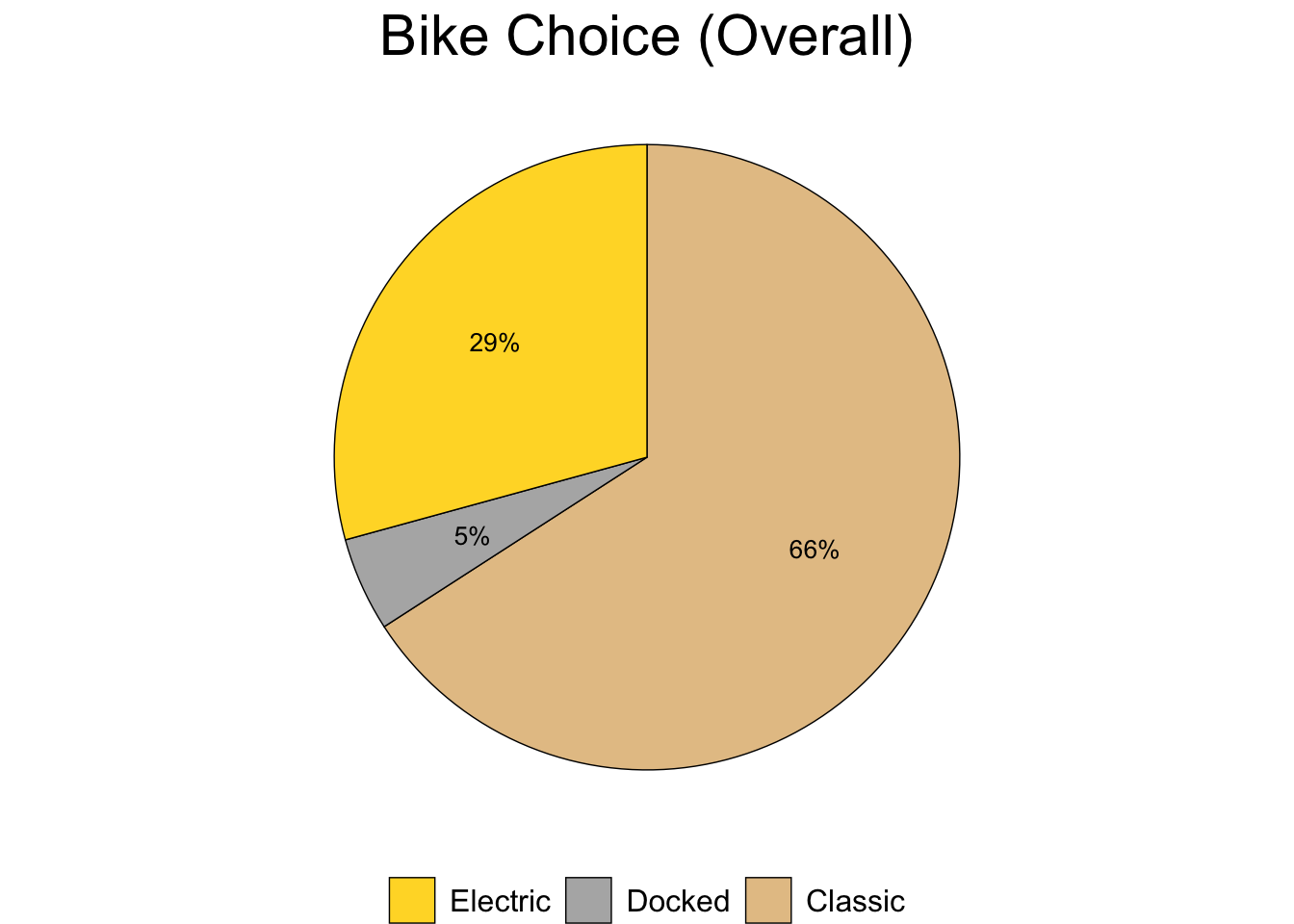
Figure 3.11: Total Bike Choice
# Bar chart: member vs. casual, bike choice
bike_data %>%
  select(rideable_type, member_casual) %>%
  group_by(rideable_type, member_casual) %>%
  count(rideable_type) %>%
  ggplot(aes(x = member_casual, y = n, fill = rideable_type)) +
    geom_col() +
    geom_text(aes(label = comma(n)),
              position = position_stack(vjust =0.5), size = 3) +
    scale_y_continuous(labels = comma) +
    scale_fill_manual(values = c("#E5C494", "#B3B3B3", "#FFD92F"), name = "Bike Type",
                      labels = c("Classic", "Docked", "Electric")) +
    labs(title = "Bike Choice: Casuals vs. Members", x = "", y = "Number of Rides\n") +
    theme(legend.title = element_blank(), legend.key.size = unit(0.65, "cm"),
          legend.text = element_text(size = 12), axis.text.x = element_text(size = 14),
          plot.title = element_text(color = "black", size = 22))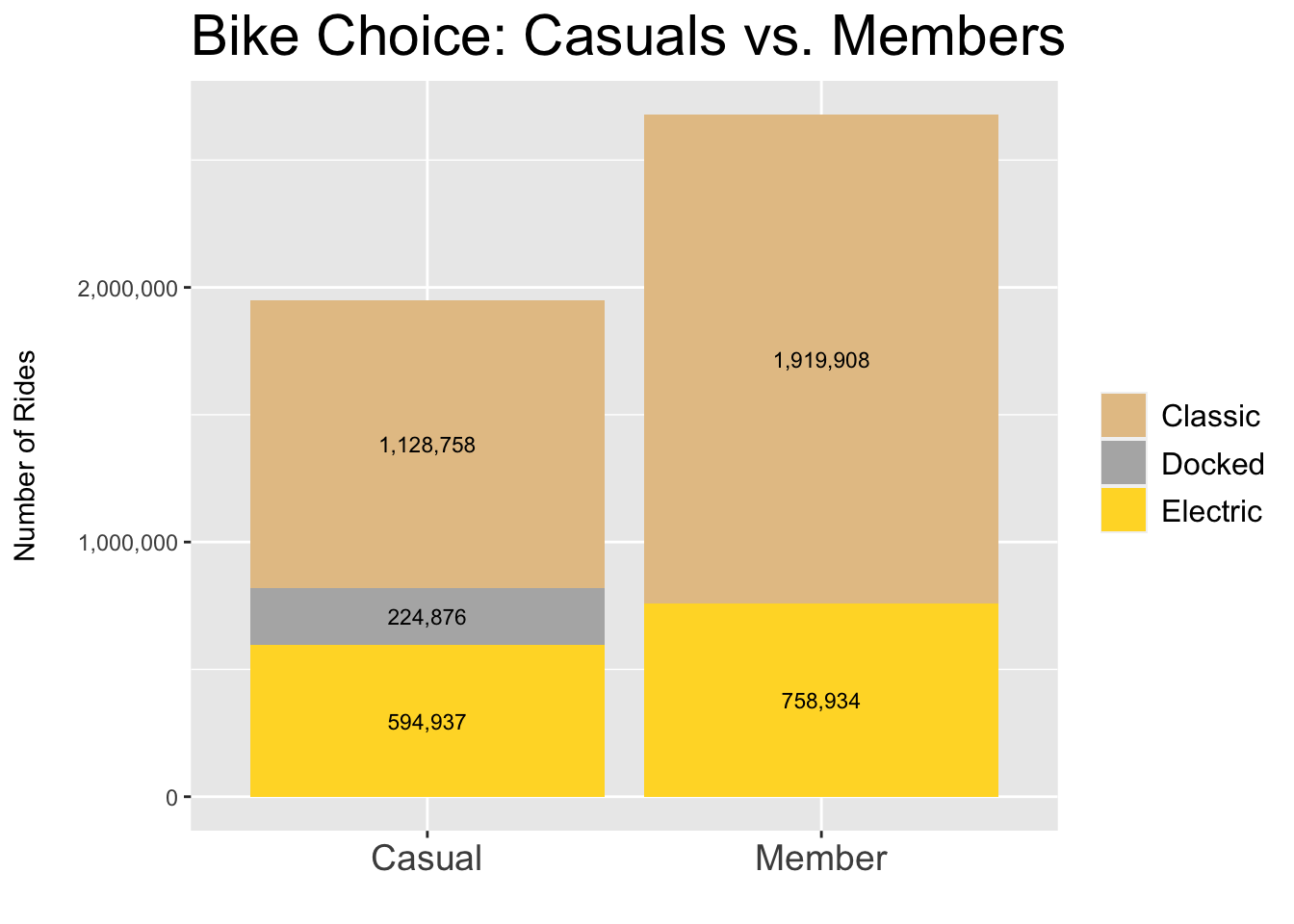
Figure 3.12: Casual vs. Member - Choice
# Pie chart: types of bikes
bike_data %>%
  select(rideable_type, member_casual) %>%
  group_by(member_casual) %>%
  count(rideable_type) %>%
  mutate(perc = percent(n/sum(n))) %>%
  ggplot(aes(x = "", y = n, fill = rideable_type)) +
    geom_bar(stat = "identity", size = 0.25, color = "black", position = "fill") +
    coord_polar(theta = "y", direction = -1) +
    facet_wrap( ~ member_casual) +
    geom_text(aes(x = 1.05, label = perc), position = position_fill(vjust=0.5)) +
    theme_void() +
    scale_fill_manual(name = "", values = c("#E5C494", "#B3B3B3", "#FFD92F"),
                      labels = c("Classic", "Docked", "Electric")) +
    labs(title = "Bike Choice\n") +
    theme(legend.title = element_blank(), legend.key.size = unit(0.65, "cm"),
          legend.text = element_text(size = 12), legend.position = "bottom",
          strip.text.x = element_text(size = 14),
          plot.title = element_text(color = "black", size = 22, hjust = 0.5)) +
    guides(fill = guide_legend(reverse = TRUE, title.position = "top"))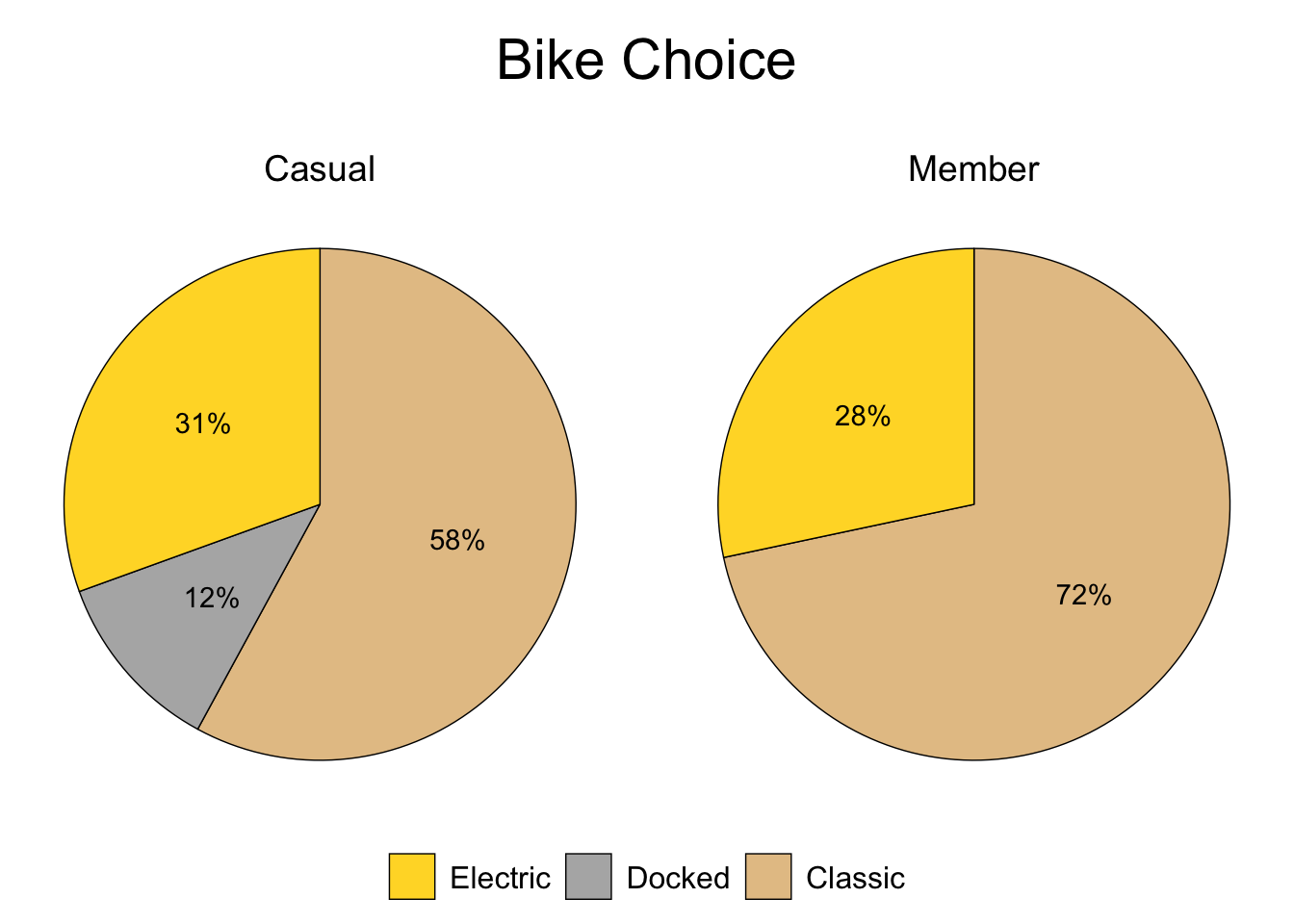
Figure 3.13: (Pie) Casual vs. Member - Choice
# Bar Chart: rideable_type / day
bike_data %>%
  select(trip_day, rideable_type, member_casual) %>%
  group_by(trip_day, rideable_type, member_casual) %>%
  count(rideable_type) %>%
  ggplot(aes(x = member_casual, y = n, fill = rideable_type)) +
    geom_col() +
    facet_wrap(~ trip_day) +
    scale_y_continuous(labels = comma) +
    scale_fill_manual(values = c("#E5C494", "#B3B3B3", "#FFD92F"),
                      labels = c("Classic", "Docked", "Electric")) +
    labs(title = "Bike Choice: Casuals vs. Members", subtitle = "Days of the Week",
         x = "", y = "Number of Rides\n") +
    theme(legend.title = element_blank(), legend.key.size = unit(0.5, "cm"),
          legend.text = element_text(size = 10),
          plot.title = element_text(color = "black", size = 22))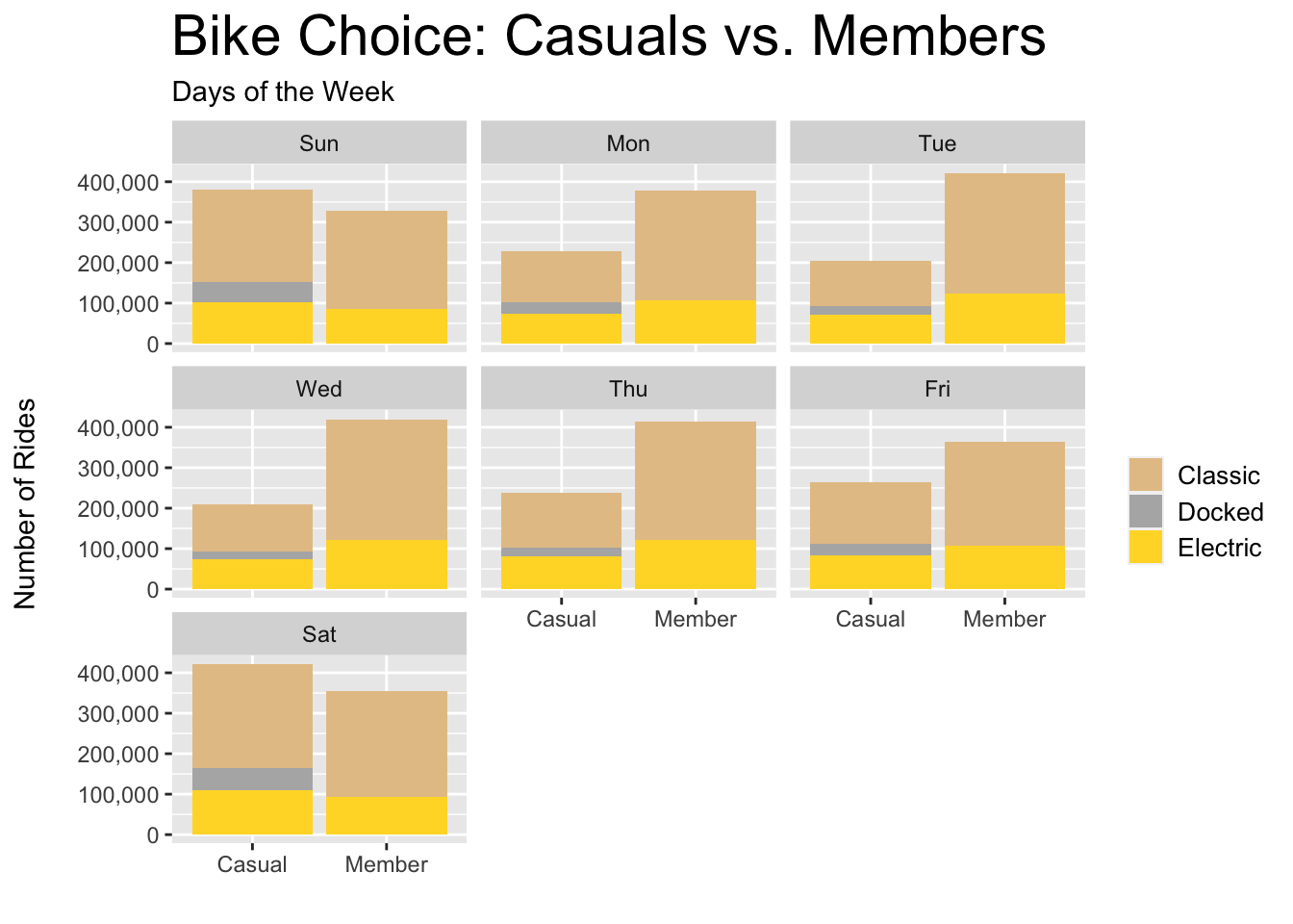
Figure 3.14: Casual vs. Member - Choice per Day
# Bar chart: bike type choice member vs. casual, by month
bike_data %>%
  select(trip_month, rideable_type, member_casual) %>%
  group_by(trip_month, rideable_type, member_casual) %>%
  count(rideable_type) %>%
  ggplot(aes(x = member_casual, y = n, fill = rideable_type)) +
    geom_col() +
    facet_wrap(~ trip_month) +
    scale_y_continuous(labels = comma) +
    scale_fill_manual(values = c("#E5C494", "#B3B3B3", "#FFD92F"),
                      labels = c("Classic", "Docked", "Electric")) +
    labs(title = "Bike Choice: Casuals vs. Members", subtitle = "Months of the Year",
         x = "", y = "Number of Rides\n") +
    theme(legend.title = element_blank(), legend.key.size = unit(0.5, "cm"),
          legend.text = element_text(size = 10),
          plot.title = element_text(size = 22))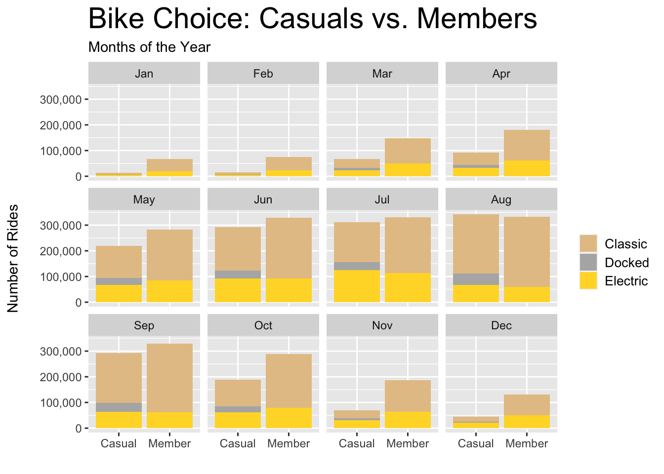
Figure 3.15: Casual vs. Member - Choice per Month
3.4.4 Viz: Popular Routes
# Top 10 routes member vs. casual
popular_routes <- bike_data %>%
                    select(route, member_casual) %>%
                    group_by(route, member_casual) %>%
                    count(route) %>%
                    arrange(member_casual, desc(n)) %>%
                    group_by(member_casual) %>%
                    slice(1:10)
# Bar Chart: Top 10 routes casual
popular_routes %>%
filter(member_casual == "Casual") %>%
mutate(order = rank(route)) %>%
ggplot(aes(x = reorder(route, n), y = n)) +
geom_col(aes(fill = reorder(route, -n)), position = "dodge") +
scale_y_continuous(labels = comma) +
geom_text(aes(y = 1200, label = n), size = 3) +
labs(title = "Top 10 Popular Routes for Casual Riders\n",
x = "", y = "Number of Rides") +
theme(panel.background = element_blank(), legend.title = element_text(size = 10),
plot.title = element_text(size = 22, hjust = 1.2),
legend.direction = "vertical", legend.text = element_text(size = 8),
legend.key.size = unit(0.5, "cm"), legend.position = "none") +
coord_flip() +
scale_fill_manual(name = "Route Name",
values = colorRampPalette(brewer.pal(8,"Set2"))(10))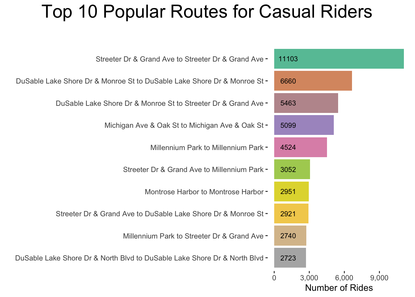
Figure 3.16:
# Pie Chart: Top 10 routes casual
popular_routes %>%
  filter(member_casual == "Casual") %>%
  mutate(perc = percent(n/sum(n), accuracy = 0.1)) %>%
  ggplot(aes(x = 1, y = n, fill = reorder(route, -n))) +
    geom_col(color = "black", size = 0.2, position = "stack", orientation = "x") +
    geom_text(aes(x = 1.25, label = perc),
              position = position_stack(vjust = 0.5), size = 2.5) +
    coord_polar(theta = "y", direction = -1) +
    theme_void() +
    labs(title = "Top 10 Popular Routes for Casual Riders\n",
         x = "", y = "Number of Rides") +
    theme(plot.title = element_text(size = 22, hjust = -0.25),
          legend.title = element_blank(), legend.text = element_text(size = 8),
          legend.key.size = unit(0.45, "cm")) +
    scale_fill_manual(name = "Route Name",
                      values = colorRampPalette(brewer.pal(8,"Set2"))(10))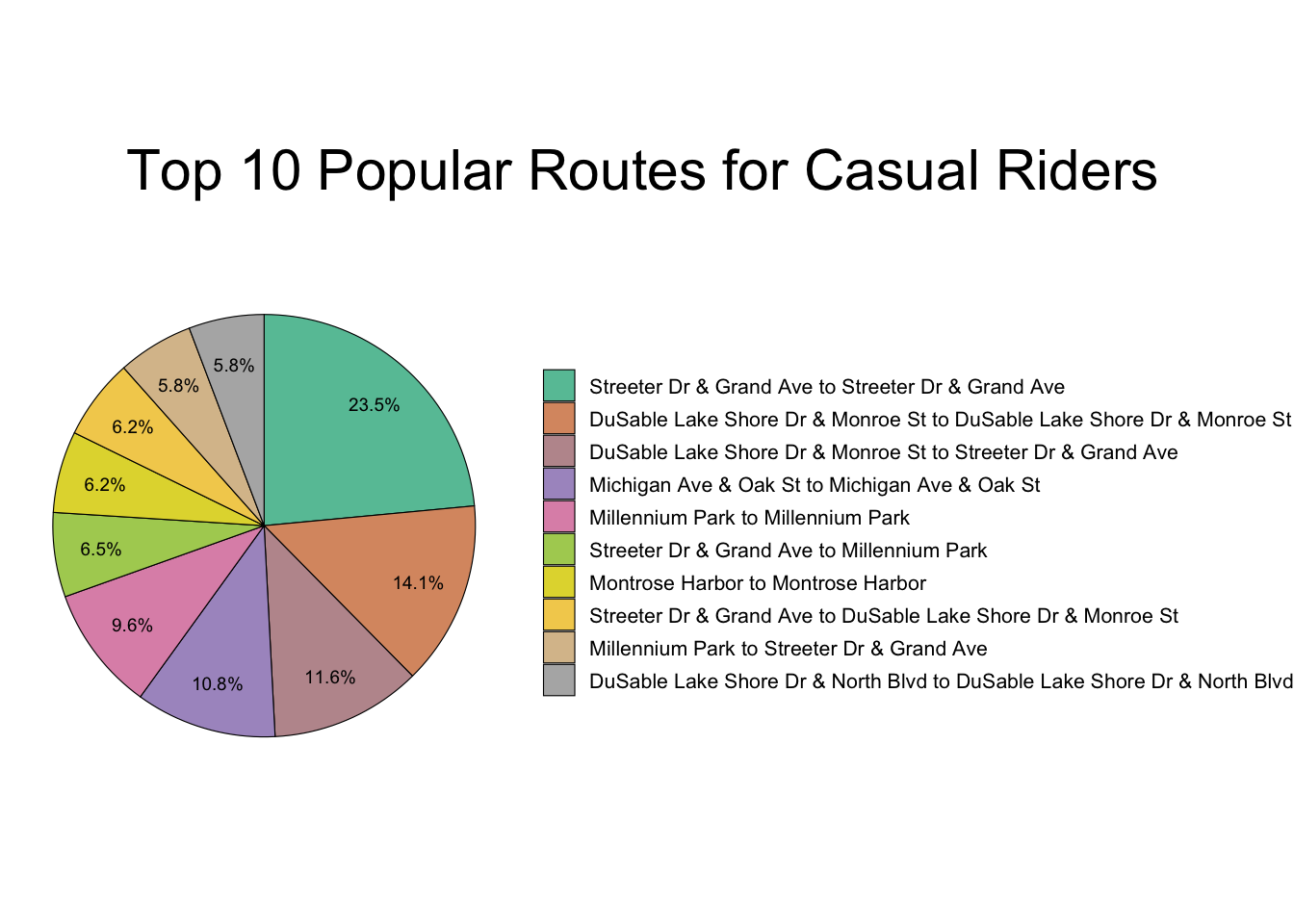
Figure 3.17:
# Bar Chart: Top 10 routes member
popular_routes %>%
  filter(member_casual == "Member") %>%
  mutate(order = rank(route)) %>%
  ggplot(aes(x = reorder(route, n), y = n)) +
    geom_col(aes(fill = reorder(route, -n)), position = "dodge") +
    scale_y_continuous(labels = comma) +
    geom_text(aes(y = 375, label = n), size = 3) +
    labs(title = "Top 10 Popular Routes for Annual Members\n",
         x = "", y = "Number of Rides") +
    theme(panel.background = element_blank(), legend.title = element_text(size = 12),
          plot.title = element_text(size = 22, hjust = 1.25),
          legend.text = element_text(size = 10), legend.position = "none",
          legend.key.size = unit(0.75, "cm")) +
    coord_flip() +
    scale_fill_brewer(name = "Route Name", palette = "Set3")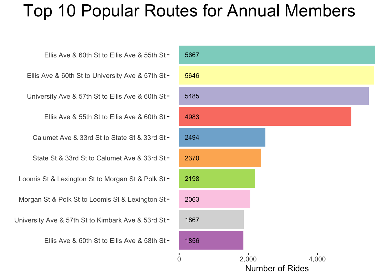
Figure 3.18:
# Pie Chart: Top 10 routes member
popular_routes %>%
  filter(member_casual == "Member") %>%
  mutate(perc = percent(n/sum(n), accuracy = 0.1)) %>%
  ggplot(aes(x = 1, y = n, fill = reorder(route, -n))) +
    geom_col(color = "black", size = 0.2, position = "stack", orientation = "x") +
    geom_text(aes(x = 1.25, label = perc),
              position = position_stack(vjust = 0.5), size = 3) +
    coord_polar(theta = "y", direction = -1) +
    theme_void() +
    labs(title = "Top 10 Popular Routes for Annual Members\n",
         x = "", y = "Number of Rides") +
    theme(plot.title = element_text(size = 22, hjust = -0.25),
          legend.title = element_blank(), legend.text = element_text(size = 10),
          legend.key.size = unit(0.65, "cm")) +
    scale_fill_brewer(palette = "Set3")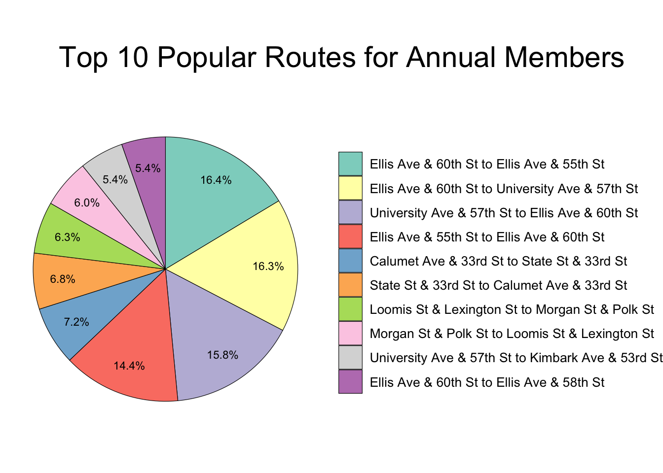
Figure 3.19:
# Join geo data
popular_routes <- popular_routes %>%
                    inner_join(bike_data %>%
                                 select(route, start_lat:end_lng, member_casual),
                                 by = c("member_casual", "route")) %>%
                    distinct(route, .keep_all = TRUE) %>%
                    group_by(member_casual) %>%
                    mutate(rank = order(order(n, decreasing=TRUE)))

# Import map of Chicago
chicago <- get_stamenmap(bbox = c(left = -87.75, bottom = 41.7,
                                  right = -87.5, top = 41.95),
                         zoom = 11)
casual_map <- ggmap(chicago, darken = 0.5) +
stat_density2d(data = filter(popular_routes, member_casual == "Casual"),
aes(x = start_lng, y = start_lat,
fill = ..level.., alpha = ..level..),
geom = "polygon", bins = 10) +
stat_density2d(data = filter(popular_routes, member_casual == "Casual"),
aes(x = end_lng, y = end_lat,
fill = ..level.., alpha = ..level..),
geom = "polygon", bins = 10) +
scale_fill_gradient(low = "green", high = "red") +
scale_alpha(range = c(0, 0.75), guide = "none") +
labs(title = "Casual Rider Hotspot", x = "", y = "") +
theme(legend.position = "none", plot.title = element_text(size = 16),
axis.ticks = element_blank(), axis.text = element_blank())
member_map <- ggmap(chicago, darken = 0.5) +
stat_density2d(data = filter(popular_routes, member_casual == "Member"),
aes(x = start_lng, y = start_lat,
fill = ..level.., alpha = ..level..),
geom = "polygon", bins = 10) +
stat_density2d(data = filter(popular_routes, member_casual == "Member"),
aes(x = end_lng, y = end_lat,
fill = ..level.., alpha = ..level..),
geom = "polygon", bins = 10) +
scale_fill_gradient(low = "green", high = "red") +
scale_alpha(range = c(0, 0.75), guide = "none") +
labs(title = "Annual Member Hotspot", x = "", y = "") +
theme(legend.position = "none", plot.title = element_text(size = 16),
axis.ticks = element_blank(), axis.text = element_blank())
grid.arrange(casual_map, member_map, nrow = 1)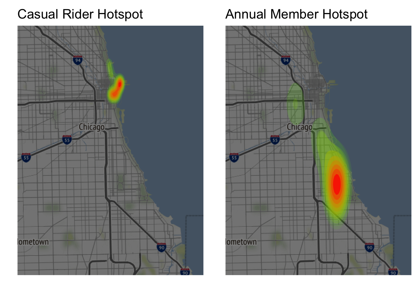
Figure 3.20: Heatmaps Based on Popular Routes
3.5 Share & Act (Final Report)
3.5.1 Key Observations
Figure 3.1 shows that the target group – casual riders – is 42% of total users.
Figures 3.2 and 3.3 show that 54.7% of total casual rides are taken during the weekend.
Offer a membership program tailored towards discounted weekend use with incentive(s) to upgrade to an annual membership.
Figures 3.4 and 3.5 show that almost half of the total casual rides are taken during the summer.
Offer a summer membership program with incentive(s) to upgrade to an annual membership.
Figures 3.6 and 3.7 show that casual riders tend to take trips during summer afternoons, suggesting that the target demographic is not likely to be students or commuters.
- Students and commuters would show higher use during off-seasons, as well as mornings and weekdays - as is shown by members in Figures 3.6 and 3.8
Figure 3.20 shows that casual riders take the most trips in Downtown Chicago (see Figure 3.16 for popular route names).
Allocate more resources towards marketing in Downtown Chicago (The Loop).
Figures relevant to bike choice (3.11 - 3.15) indicate that casual riders and annual members exhibit similar behavior; however, it’s worth investigating why 12% of casual riders use a docked bike when 0% of members do.