Chapter 5 NN: XOR [ML|PY,MATH]

5.1 Backpropagation and XOR

For my Multivariable Calculus final project, I chose to study the backpropagation algorithm in the context of a fully-connected feed-forward neural network with one hidden layer – the canonical multilayer perceptron or “vanilla” neural net.

In short, backpropagation is a machine learning technique that uses gradient descent calculus and grants neural networks the ability to perform non-linear classification tasks. I will use this learning technique to show how such a neural network is capable of learning the XOR logical gate.

5.1.1 Motivation

The XOR classification task is non-linear (not linearly separable) because it’s quite literally impossible to use a single line to separate our two groups.

In the case of XOR, the gate outputs a 1 if and only if one of the two inputs is a 1, and 0 otherwise.

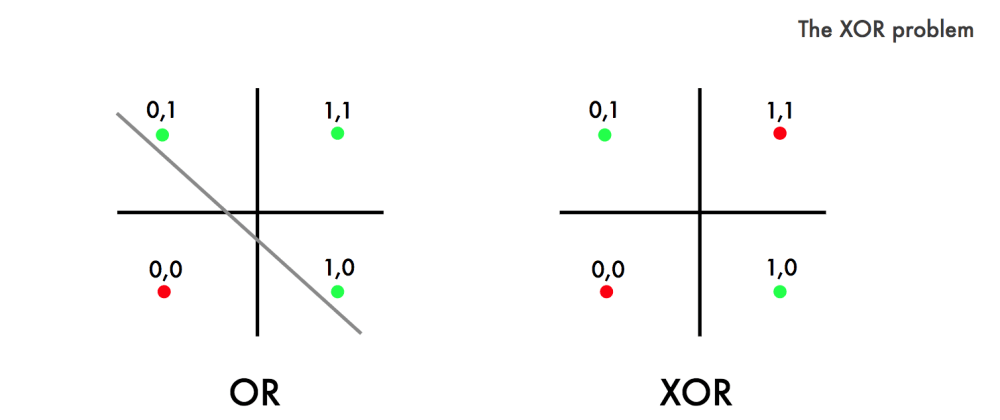
Figure 5.1: Linear vs. Nonlinear Classification (Google Images)

Referencing the right side of Figure 5.1 above, the two groups we have to classify for this case are:

When it should output a 1 (labeled as a green dot)
When it should output a 0 (labeled as a red dot)

If the XOR classification task were linear, we would be able to separate the green dots from the red dots with a single line (as we do with OR).

Aside

As a side note, focusing on the XOR case allows us to ignore the confusing notation that naturally comes with the generalized form of neural networks – and although I love linear algebra – it is only a distraction in a case as simple as this; therefore, the use of explicit notation and the stripping of linear algebra will make the learning curve towards understanding the heart of such a profound machine learning technique a lot less steep.

Additionally, the XOR problem is a particularly famous one in neural networks, and I recommend anyone interested to read how XOR helped develop (and almost “destroyed”) the field of neural networks in its infancy. See “Explained: Neural Networks” or the 2017 forward to Perceptrons (Minsky & Papert, 1969/1988).

5.2 Activation

Since this situation isn’t linear (as it is with most natural phenomena), we introduce a non-linearity – or activation function – into the network to avoid it calculating linear combinations of values as if it were a linear classification task.

This is what allows our neural network to successfully begin learning such non-linear phenomena, thus giving it the capability to perform non-linear classification.

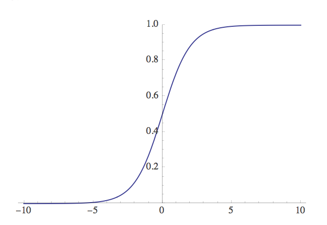
Figure 5.2: The sigmoid activation function plotted in Mathematica.

We use a sigmoidal activation function (Figure 5.2) to squash and map our inputs to the range $(0,1)$ .

This function also serves as an abstract representation of the action potential process that takes place during the firing in a neuron: $\varphi(x) = \frac{1}{1+e^{-x}}; \quad \varphi(x) \colonequals \varphi_x$

which has a neat derivative of: $\varphi_x (1 - \varphi_x).$

5.3 Multivariable Calculus

The cost function, or error of this network, which we want to minimize is: $E = \frac{1}{2}(y - \hat y)^2 \tag{1}$ where $y$ is the correct output and $\hat y$ is the network’s output.

To minimize our error, we have to adjust each of the network’s weights until we get the desired output. This is done through backpropagation, using the negative gradient to find the steepest descent towards the local minimum of the error for each weight.

Referencing Figure 5.3, this gradient is defined as a vector whose indices are the rate of change in the direction of steepest descent for every weight: $- \nabla E \equiv - \left[ \frac{\partial E}{\partial w_1}, \frac{\partial E}{\partial w_2}, \frac{\partial E}{\partial w_{11}}, \ldots , \frac{\partial E}{\partial w_{22}} \right] \tag{2.1}$

We use the training rule defined as follows to update all of our weights (defined here generally as $w$ ) using the corresponding gradient index which holds that specific weight: $\Delta w = - \alpha \frac{\partial E}{\partial w}; \quad \alpha \in (0,1)$ where $\alpha$ is the learning rate, or how fast the algorithm will try to approach the local minimum.

5.3.1 Dissecting the Network

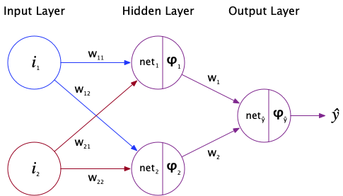
Figure 5.3: XOR Neural Network Diagram that I made in OmniGraffle.

With the visual aid above, this entire network can be defined as follows: $\begin{align*} \hat y &= \varphi(\text{net}_{\hat y})\\ \text{net}_{\hat y} &= \varphi(\text{net}_1)w_1 + \varphi(\text{net}_2)w_2\\ \text{net}_1 &= i_1w_{11} + i_2w_{21}\\ \text{net}_2 &= i_1w_{12}+i_2w_{22} \end{align*}$

This notation will be used when computing the partial derivatives, as to avoid confusion between what is a function and what is multiplication: $\begin{align*} \varphi(\text{net}_{\hat y}) \coloneqq \varphi_{\hat y}\\ \varphi(\text{net}_1) \coloneqq \varphi_1\\ \varphi(\text{net}_2) \coloneqq \varphi_2 \end{align*}$

Since this is a multivariable function, we have to apply the chain rule to take into account everything that’s a function of the hidden layer weights: $\Delta w_{\hat y} = - \alpha \frac{\partial E}{\partial w_{\hat y}} = - \alpha \frac{\partial E}{\partial \hat y} \frac{\partial \hat y}{\partial \text{net}_{\hat y}} \frac{\partial \text{net}_{\hat y}}{\partial w_{\hat y}} \tag{2.2}$

Equation 2.2 will be used for the proposed adjustments of these two weights, $w_{\hat y} \in \{ w_1, w_2\}$ , which are directly connected to the output node where the partials are: $\begin{align*}\\ \frac{\partial E}{\partial \hat y} &= \frac{\partial}{\partial \hat y} \left(\frac{1}{2}(y - \hat y)^2\right) = -(y - \hat y)\\\\ \frac{\partial \hat y}{\partial \text{net}_{\hat y}} &= \frac{\partial}{\partial \hat y} \Bigl(\varphi_{\hat y}\Bigr) = \varphi_{\hat y}(1-\varphi_{\hat y})\\\\ \frac{\partial \text{net}_{\hat y}}{\partial w_{\hat y}} &= \frac{\partial}{\partial w_{\hat y}} \Bigl(\varphi_1w_1 + \varphi_2w_2\Bigr) = \varphi_1 \text{ \ or \ } \varphi_2\\ \\&\therefore&\\\\ \Delta w_1 &= \alpha(y - \hat y)\varphi_{\hat y}(1-\varphi_{\hat y})\varphi_1 \\ \Delta w_2 &= \alpha(y - \hat y)\varphi_{\hat y}(1-\varphi_{\hat y})\varphi_2 \end{align*}$
The only noticeable difference between these two weight changes is which net input was activated prior to it. Thus begins our backpropagation!

For the four weights directly connected to the input nodes we have to extend the chain rule even further to account for everything that’s a function of the inputs: $\Delta w_{ij} = - \alpha \frac{\partial E}{\partial w_{ij}} = {\color{teal} - \alpha \frac{\partial E}{\partial \hat y} \frac{\partial \hat y}{\partial \text{net}_{\hat y}} \frac{\partial \text{net}_{\hat y}}{\partial w_{\hat y}}} \frac{\partial w_{\hat y}}{\partial \text{net}_i} \frac{\partial \text{net}_i}{\partial w_{ij}}$ where $w_{ij}$ represents the $j^{th}$ weight directly connected to the $i^{th}$ input.

Using Equation 2.2 associated with the above colored text simplifies this to: $\Delta w_{ij} = \Delta w_{\hat y} \frac{\partial w_{\hat y}}{\partial \text{net}_i} \frac{\partial \text{net}_i}{\partial w_{ij}} \tag{2.3}$

Equation 2.3 will be used for the proposed adjustments of these four weights which are directly connected to the input node, namely $w_{ij} \in \{w_{11},w_{12},w_{21},w_{22} \}$ .

Basically, we’re looking at each of the four paths that need to be taken in order to reach the original inputs with our starting point being our output (as color-coded in Figure 5.3). Recall that: $\begin{align*} \text{net}_1 &= i_1w_{11}+i_2w_{21}\\ \text{net}_2 &= i_1w_{12}+i_2w_{22} \end{align*}$

Additionally, since the weights connected to the output neuron are influenced by their respective activated net inputs:

$\begin{align*} \frac{\partial w_{\hat y}}{\partial \text{net}_i} &= \frac{\partial}{\partial \text{net}_i} \left(\varphi_i\right) = \varphi_i(1 - \varphi_i)\\\\ &\therefore&\\\\ \Delta w_{11} &= \Delta w_1 \ \varphi_1(1-\varphi_1)i_1\\ \Delta w_{12} &= \Delta w_2 \ \varphi_2(1-\varphi_2)i_1\\ \Delta w_{21} &= \Delta w_1 \ \varphi_1(1-\varphi_1)i_2\\ \Delta w_{22} &= \Delta w_2 \ \varphi_2(1-\varphi_2)i_2\\ \end{align*}$

The noticeable differences between these four weight changes are the actual input itself in conjunction with which hidden node the weight’s attached to.

5.4 Conclusion

Focusing on the XOR case to start, as opposed to tackling the generalized form of neural networks, provides a more easily-digestible intuition for how backpropagation works in neural networks. The network literally propagates backward along every possible path connecting the output node to the input nodes in order to discover the right values for each individual weight.

Over multiple gradient descent iterations, this network will successfully converge towards a local minimum of the multivariable error function, therefore learning the XOR gate. This means that you could input any combination of two binary numbers and it would successfully return the correct XOR response to such inputs without looking up a hard-coded truth table.

This non-linear classification task was previously impossible for feed-forward networks due to their inherently linear structure. Without the invention of the backpropagation algorithm, neural networks would’ve been completely disregarded only a few years after their inception. Within the last decade, the immense strides in neural networks gave birth to a technique called deep learning, now implemented within almost every cutting-edge artificial intelligence system imaginable.

5.5 Learning XOR in TensorFlow

The truth table for XOR is as follows:

\begin{array}{cc|c} A & B & A \oplus B\\ \hline 0 & 0 & 0\\ 0 & 1 & 1\\ 1 & 0 & 1\\ 1 & 1 & 0\\ \end{array}

The model adjusts its weights and converges to the truth table over the training iterations, as displayed in the output below.

# Neural Network (NN) in TensorFlow that learns the XOR gate
# Edit 2022: load older tf for old code
import tensorflow.compat.v1 as tf
tf.disable_v2_behavior()

# Sigmoid activation function

## WARNING:tensorflow:From /usr/local/lib/python3.10/site-packages/tensorflow/python/compat/v2_compat.py:107: disable_resource_variables (from tensorflow.python.ops.variable_scope) is deprecated and will be removed in a future version.
## Instructions for updating:
## non-resource variables are not supported in the long term

def activate(nodes, weights):
    net = tf.matmul(nodes, weights)
    return tf.nn.sigmoid(net)

# XOR truth table
X_XOR = [[0,0],[0,1],[1,0],[1,1]]
Y_XOR = [[0],[1],[1],[0]]

# NN parameters
N_STEPS       = 250000
HIDDEN_NODES  = 2
INPUT_NODES   = 2
OUTPUT_NODES  = 1
LEARNING_RATE = 0.05

# NN I/O
x_nn = tf.placeholder(tf.float32, shape=[len(X_XOR), INPUT_NODES])
y_nn = tf.placeholder(tf.float32, shape=[len(X_XOR), OUTPUT_NODES])

# Randomized NN weights for input layer and hidden layer
w_i = tf.Variable(tf.random_uniform([INPUT_NODES, HIDDEN_NODES], 0, 1))
w_h = tf.Variable(tf.random_uniform([HIDDEN_NODES, OUTPUT_NODES], 0, 1))

# Forward Pass through the layers
hidden = activate(x_nn, w_i)
output = activate(hidden, w_h)

# Cost function (MSE) and Backpropagation
cost = tf.reduce_mean(tf.square(Y_XOR - output))
backprop = tf.train.GradientDescentOptimizer(LEARNING_RATE).minimize(cost)

# Feed dictionary of truth table
dict_xor = {x_nn: X_XOR, y_nn: Y_XOR}

init = tf.global_variables_initializer()
sess = tf.Session()
sess.run(init)

for i in range(N_STEPS+1):
    sess.run(backprop, feed_dict=dict_xor)
    if i in [0, 25000, 50000, 100000, 250000]:
        print("--------------------")
        print("Iteration", i, "Guess:",
              sess.run(tf.transpose(output), feed_dict=dict_xor), "\n")
        print("Input Weights:\n", sess.run(w_i))
        print("Hidden Weights:\n", sess.run(w_h), "\n")
        print("Error:", sess.run(cost, feed_dict=dict_xor))

## --------------------
## Iteration 0 Guess: [[0.6382959  0.67482334 0.68818045 0.712769  ]] 
## 
## Input Weights:
##  [[0.78813964 0.86214846]
##  [0.13670845 0.91594166]]
## Hidden Weights:
##  [[0.45105302]
##  [0.68489796]] 
## 
## Error: 0.27960813
## --------------------
## Iteration 25000 Guess: [[0.2687148  0.68361616 0.68345094 0.408158  ]] 
## 
## Input Weights:
##  [[0.7330665  4.97169   ]
##  [0.73106855 4.907222  ]]
## Hidden Weights:
##  [[-8.683456 ]
##  [ 6.6811504]] 
## 
## Error: 0.109775655
## --------------------
## Iteration 50000 Guess: [[0.15894006 0.7772046  0.77719414 0.29180697]] 
## 
## Input Weights:
##  [[0.8214333 6.0759916]
##  [0.8212353 6.054871 ]]
## Hidden Weights:
##  [[-15.087451]
##  [ 11.755179]] 
## 
## Error: 0.052423377
## --------------------
## Iteration 100000 Guess: [[0.09161668 0.8497939  0.8497923  0.19840614]] 
## 
## Input Weights:
##  [[0.87447494 6.8183227 ]
##  [0.8744301  6.8081775 ]]
## Hidden Weights:
##  [[-21.539515]
##  [ 16.951408]] 
## 
## Error: 0.023220709
## --------------------
## Iteration 250000 Guess: [[0.04534886 0.9112044  0.9112041  0.11809696]] 
## 
## Input Weights:
##  [[0.91362447 7.478241  ]
##  [0.9136126  7.4730563 ]]
## Hidden Weights:
##  [[-29.468285]
##  [ 23.374363]] 
## 
## Error: 0.007943195